 So so long
Some formulas to make working in Excel easier
If you’re used to programming in R or Python and suddenly have to do everything in Excel due to client requirements or something, you may repeatedly find yourself wondering “How do I do this thing I always do? Shouldn’t it be easy?”. Well the answer likely is no, it isn’t as easy as it should be, but yes, there is a way. Here’s a few of them that I couldn’t google for that easily.
Checking a cell for the presence of one of multiple partial text string matches
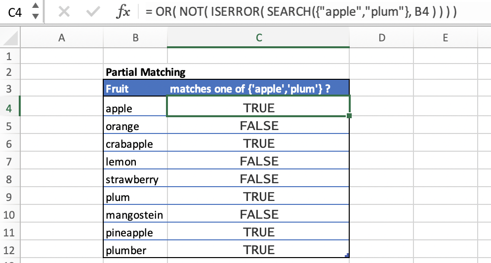
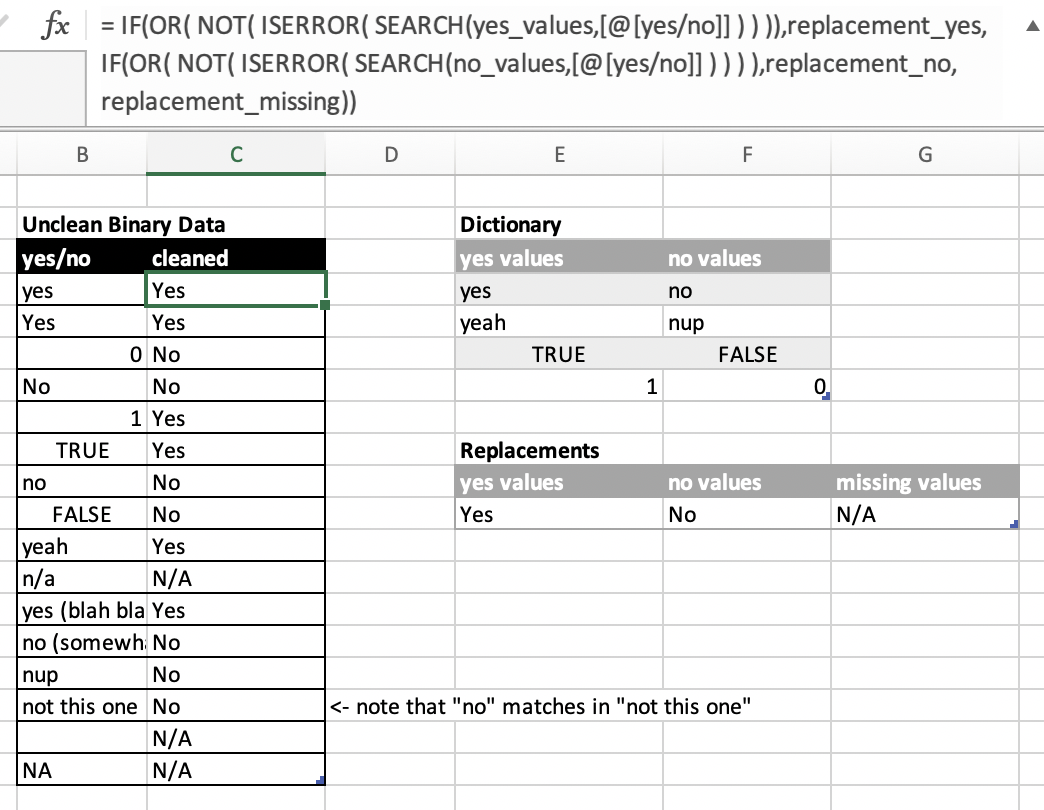
Say the data has been entered really non-uniformly. Sometimes it says ‘Yes’, sometimes it’s a 1 etc. like in the following table:
| Yes value | No value | Missing data |
|---|---|---|
| Yes | No | n/a |
| Yes (unneccesary details) | No (unneccesary details) | - |
| 1 | 0 | |
| I think so | Not this time | NA |
Any cell can contain one of these options and the unnecesary details might change. So really you want to search for a list of items and if any appear, mark it as true.
Example code to search any of the ‘Yes’ values and recode them as TRUE:
= OR( NOT( ISERROR( SEARCH({ "Yes" , "1" , "I think so" } , cell_to_search ) ) ) )
How does it work?
- This is feeding a cell array of possible yes values
{ "Yes" , "1" , "I think so" }into the search function along with the cell to search. This will output a cell array which contains a 1 where it matched the search string, and a #VALUE error where it didn’t, for example if the cell contents was “Yes blah”, it will return{1, #VALUE, #VALUE} - The
ISERROR()function will turn this into true/false values e.g.{FALSE, TRUE, TRUE} - The
NOT()function negates it to{TRUE, FALSE, FALSE} - The
OR()function concatenates it appropriately to a singleTRUEvalue output.
You can then nest some if statements to match both yes and no, leaving everything else as missing.
Finding the unique elements in an array
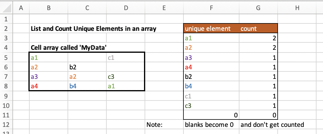
If you want to find the unique elements in a column and return them sorted, it’s easy. Just use =SORT(UNIQUE(cells)). However if you want to do this for values occuring across multiple columns in an array, it’s annoying.
First, select your array and give it a name, e.g. MyArray. Then, use this horrible formula:
=SORT(UNIQUE(INDEX(MyArray,1+INT((ROW(INDIRECT("1:"&COLUMNS(MyArray)*ROWS(MyArray)))-1)/COLUMNS(MyArray)),MOD(ROW(INDIRECT("1:"&COLUMNS(MyArray)*ROWS(MyArray)))-1+COLUMNS(MyArray),COLUMNS(MyArray))+1)))
How does it work? Lets break it into parts:
- Array element iterator
ROW(INDIRECT("1:"&COLUMNS(MyArray)*ROWS(MyArray))). Using the formula=ROW(INDIRECT("1:10"))will give me a cell array of{1;2;3;4;5;6;7;8;9;10}. So to get an iterator to go through all the elements in the array, I useROW(INDIRECT("1:"&COLUMNS(MyArray)*ROWS(MyArray))). Let’s call this iteratorinow. - Indexing the array
INDEX(array, row, column)will pull out an element of the array. so we do appropriate modulo arithmatic on the iteratorito get the column number -MOD(i-1+COLUMNS(MyArray),COLUMNS(MyArray))+1, and take the floor of a division (using theINT()function) to get the row number as row =1+INT((i-1)/COLUMNS(MyArray)). So we getINDEX(MyArray,1+INT((i-1)/COLUMNS(MyArray)),MOD(i-1+COLUMNS(MyArray),COLUMNS(MyArray))+1) - Now we have a vertical array/column (let’s call it
col) containing all the data which was in the array. We just have to applySORT(UNIQUE(col))to get out only the unique elements, and sorted in alphabetical order.
My mind went blank
- Referencing the contents of a cell will return the contents of the cell, unless it is blank. A blank cell will turn into a zero. Thus missing data can magically turn into non-missing data in the middle of your analysis. Instead of
=cell_refuse=if(isblank(cell_ref),"",cell_ref)to keep blanks blank.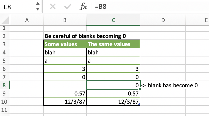
Blanks can sneakily turn into the number zero - Checking if a cell is blank using
isblank(cell_ref)will return false if the cell contains a formula which returns a blank string as a value. In this case usecell_ref=""instead.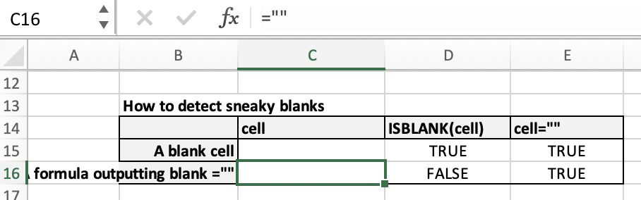
Blanks can sneakily avoid detection if they are the result of a formula
Examples
In the file excel_formulas_example.xlsx are examples of the things described above.
Dr. Gordon McDonald
Informatics Team Lead
My research interests include data science for public good, quantum physics and psychology.